¿Cómo se condiciona en una tabla dinámica?

How do you condition in a pivot table?

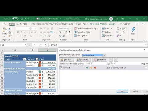
The Right Way to Apply Conditional Formatting to a Pivot Table

1. Select the data on which you want to apply conditional formatting.
2. Go to Home –> Conditional Formatting –> Top/Bottom Rules –> Above Average.
3. Specify the format (I am using “Green Fill with Dard Green Text”).
4. Click Ok.

To turn on Enable Selection:

1. Select a cell in the pivot table, and on the Ribbon, click the Options tab.
2. In the Actions group, click Select.
3. Check to see if Enable Selection is ON or OFF, as shown in the screen shot below.
4. If Enable Selection is OFF, click it to activate the feature.

When you summarize numerical data using a PivotTable, Excel displays the values with either no formatting, which can make the numbers difficult to interpret, or using a number format.

Setting to Preserve Cell Formatting

1. Right-click a cell in the pivot table, and click PivotTable Options.
2. On the Layout & Format tab, in the Format options, remove the check mark from Autofit Column Widths On Update.
3. Add a check mark to Preserve Cell Formatting on Update.
4. Click OK.

Change the source data for a PivotTable

1. Click the PivotTable report.
2. On the Analyze tab, in the Data group, click Change Data Source, and then click Change Data Source. The Change PivotTable Data Source dialog box is displayed.
3. Do one of the following:

Pivot Table Tips

1. You can build a pivot table in about one minute.
2. Clean your source data.
3. Count the data first.
4. Plan before you build.
5. Use a table for your data to create a “dynamic range”
6. Use a pivot table to count things.
7. Show totals as a percentage.
8. Use a pivot table to build a list of unique values.

For applying conditional formatting in this pivot table, follow the below steps: 1 Select the cells range for which you want to apply conditional formatting in excel. We have selected the range B5:C14… 2 Go to the HOME tab > Click on Conditional Formatting option under Styles > Click on Highlight Cells Rules option > Click… More

To turn on Enable Selection: Select a cell in the pivot table, and on the Ribbon, click the Options tab. In the Actions group, click Select Check to see if Enable Selection is ON or OFF, as shown in the screen shot below.

Add new parameters columns with fill_value and also is possible use nunique for aggregate function: city_count = df.pivot_table (index = “Area”, values = “City”, columns=’Condition’, aggfunc = lambda x : x.nunique (), margins = True, fill_value=0) print (city_count) Condition Bad Good All Area A 2 2 4 B 0 1 1 C 0 1 1 D 0 1 1 All 2 5 7

In the Actions group, click Select Check to see if Enable Selection is ON or OFF, as shown in the screen shot below. If Enable Selection is OFF, click it to activate the feature. If Enable Selection is ON, click the worksheet, to close the menu without making a selection.