¿Cómo resalto duplicados consecutivos en Excel?

How do I highlight consecutive duplicates in Excel?

To do this, select the cells with data (not including the column header) and create a conditional formatting rule with one of the following formulas:

1. To highlight consecutive duplicates without 1st occurrences: =$A1=$A2.
2. To highlight consecutive duplicates with 1st occurrences: =OR($A1=$A2, $A2=$A3)

1. Quickly Identify Duplicates

1. Select the dataset in which you want to highlight duplicates.
2. Go to Home –> Conditional Formatting –> Highlighting Cell Rules –> Duplicate Values.
3. In the Duplicate Values dialogue box, make sure Duplicate is selected in the left drop down.
4. Click OK.

Google Sheets: How to highlight duplicates in a single column

1. Open your spreadsheet in Google Sheets and select a column.
2. For instance, select column A > Format > Conditional formatting.
3. Under Format rules, open the drop-down list and select Custom formula is.
4. Enter the Value for the custom formula, =countif(A1:A,A1)>1.

Select the range of cells, the table, or the whole sheet that you want to apply conditional formatting to. On the Home tab, click Conditional Formatting. Point to Highlight Cells Rules, and then click Duplicate Values. Next to values in the selected range, click unique or duplicate.

Go to HOME >> Styles >> Conditional Formatting >> Highlight Cells Rules and select Duplicate Values. A new window will appear. Make sure that you’ve selected Duplicate and click OK. All rows which are duplicates are now highlighted.

Find and remove duplicates

1. Select the cells you want to check for duplicates.
2. Click Home > Conditional Formatting > Highlight Cells Rules > Duplicate Values.
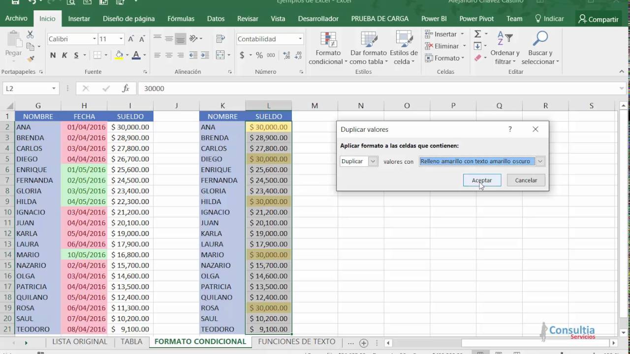
3. In the box next to values with, pick the formatting you want to apply to the duplicate values, and then click OK.

Note: Excel can’t highlight duplicates in the Values area of a PivotTable report. Click Home > Conditional Formatting > Highlight Cells Rules > Duplicate Values. In the box next to values with, pick the formatting you want to apply to the duplicate values, and then click OK.

1. Select the range with the data you want to format. 2. Create a new conditional formatting rule with clicking Conditional Formatting > New Rule under Home tab. 3. In the New Formatting Rule dialog box, you can: 1). Select Use a formula to determine which cells to format in the Select a Rule Type box; 2).

Figure 2: The rows with a duplicate value in column A are now formatted. When applying conditional formatting in this fashion the dollar signs around the cell references are critical. There’s an intangible aspect to Conditional Formatting because you’re entering one formula that needs to cover multiple rows.

Open both workbooks you will apply conditional formatting across, select a blank cell you will refer values from another workbook, says Cell G2, enter the formula =’ [My List.xlsx]Sheet1′!A2 into it, and then drag the AutoFill Handle to the range as you need.

Conditional Formatting Across Multiple Cells in Excel

1. Highlight the cell in the row that indicates inventory, our “Units in Stock” column.
2. Click Conditional Formatting.
3. Select Highlight Cells Rules, then choose the rule that applies to your needs.

Select the data range you want to color the duplicate values, then click Home > Conditional Formatting > Highlight Cells Rules > Duplicate Values.

1. Then in the popping dialog, you can select the color you need to highlight duplicates from the drop down list of values with.
2. Click OK.

You can add many conditional formats to the same cell and range in order to get the desired effect.

Note: With the above formula, you can highlight all the consecutive duplicate cells, if you want to highlight the consecutive duplicate cells without the first occurrences, please apply this formula: =$A1=$A2 in the Conditional Formatting, and you will get the following result:

However, looking closer we can see that there are some users with the same name but different IDs. This means that using the pre-defined “Duplicate Values” Conditional Formatting is not good enough in this case. Simply deleting the highlighted values based on the name criteria would result in losing data.

Color the duplicate values. 1. Select the data range you want to color the duplicate values, then click Home > Conditional Formatting > Highlight Cells Rules > Duplicate Values. See screenshot: 2. Then in the popping dialog, you can select the color you need to highlight duplicates from the drop down list of values with.

I am working with Excel 2013. I need conditional formatting dependent on a condition: If cell L2 is not empty and cell M2 is not empty format cell D2 with background color. I tried =AND ($L2>0,$M2>0) to apply to cell D2 and it works fine. Now I want cell D3 to get the rule =AND ($L3>0,$M3>0).

Finding and Highlight Duplicates in Multiple Columns in Excel

1. Select the data.
2. Go to Home –> Conditional Formatting –> Highlight Cell Rules –> Duplicate Values.
3. In the Duplicate Values dialog box, select Duplicate in the drop down on the left, and specify the format in which you want to highlight the duplicate values.

How to highlight cell rules after second occurrence

1. Select the range with duplicate values (i.e. range A1:B16 in our case).
2. Go to ‘Home’ ‘Conditional Formatting’.
3. Click on ‘New Rule’.
4. Click on ‘Use a formula to determine which cells to format’.
5. Type ‘=COUNTIF($A$1:A1,A1)>1’ in formula bar.
6. Click on the ‘Format’ button.

Here are the steps to do this:

1. Select the entire data set.
2. Click the Home tab.
3. In the Styles group, click on the ‘Conditional Formatting’ option.
4. Hover the cursor on the Highlight Cell Rules option.
5. Click on Duplicate Values.
6. In the Duplicate Values dialog box, make sure ‘Duplicate’ is selected.
7. Specify the formatting.

Highlight duplicate rows in one column Go to HOME >> Styles >> Conditional Formatting >> Highlight Cells Rules and select Duplicate Values. A new window will appear. Make sure that you’ve selected Duplicate and click OK. All rows which are duplicates are now highlighted.